PJAS and Some Catching Up – Corbin's Confounding Computers

Hello world!

So if you’re just here for the technobabble about my PJAS project, skip down a little bit, otherwise I feel it necessary to explain where the heck I’ve been. I managed to get myself stuck in a rut a few months ago, where I ended up staring at all my unfinished drafts and wondering why I even bother when I can’t finish a post (very bad thinking). Pulling myself out of this rut was somewhat a revolutionary turn in my evolution towards growth mindset thinking. To sum up the several sleepless nights, I essentially decided “improvement over time with crappy posts is better than having no consistency at all.” So expect some weird consistency for a while. This also means I’ll have a few posts pop up on some old projects, but I feel better personally if I complete those posts rather than discard them.

Without further ado, onto the sciencey-things! So back in February I competed in the regional competition for the Pennsylvania Junior Academy of Science, and won first place. So then I competed again in May at the states competition, and won first place again! (Woot woot!) … but what was the project you ask? Fantastic railroading question! I simulated and analyzed the spread of diseases using a set of differential equations.

To start I need to cover some basics of differential equations. I have not taken a calculus course yet, so take what I say from here with skepticism, but from what I understand the differential equations I use give us the instantaneous slope for a given time on a graph, and this is essentially all you need to know to implement them into Python. The equations we’ll be using are known as the SIR Model, it’s a model used for modeling disease spread and was proposed by Kermack and McKendrick in 1927. The SIR Model:

(1) $\begin{align*} \frac{dS}{dt} = -\frac{\beta I S}{N} \end{align*}$

(2) $\begin{align*} \frac{dI}{dt} = \frac{\beta I S}{N} - \gamma I \end{align*}$

(3) $\begin{align*} \frac{dR}{dt} = \gamma I \end{align*}$

The equation has a few key variables, N is the total population, S is susceptible stock, I is infected stock, and R is recovered stock. Alongside these, we also have $\beta$ and $\gamma$ . $\beta$ is the transmission rate for the disease and $\gamma$ is the recovery rate (usually 1 over the general recovery period). In order to find the transmission rate for the disease, we need to know the recovery rate and the basic reproductive number ( $R_0$ ). Now in my research for this project, I couldn’t find much on how they calculate this number, but it seems to be generally available for most diseases online. From the basic reproduction rate we can calculate our transmission rate using the following formula:

(4) $\begin{align*} R_0 = \frac{\beta}{\gamma} \end{align*}$

(5) $\begin{align*} \beta = R_0 \times \gamma \end{align*}$

That covers pretty much everything we need to know about the SIR Model, so onto the programming! For this project we’re gonna have to use SciPy, NumPy, and MatPlotLib. We’ll start off by defining the many variables we’re gonna be using here.

# Total Population
N = 7406000
# Initial infected and recovered stock
I0, R0 = 1, 0
# (R_0)
R = 15
gamma = 1/21
beta = (gamma*R)
# Total susceptible stock
S0 = N - I0 - R0

The example I’m using here is a measles outbreak in Washington state, as it’s the same example I used when I competed at the state competition. Next we create a vector of the initial conditions, we need to do this to pass it by SciPy’s Odeint function later in order to solve the differential equations. We also create a time grid using numpy, this is to represent the total time simulated and be used in our final graphing task.

t = np.linspace(0, 160)
y0 = S0, I0, R0

Now we just need one final piece, the actual equations. In order to pass them through SciPy it’s easiest if we have them inside their own function. We just implement them as normal equations using the standard operators.

def SIR(y, t, N, beta, gamma):
    S, I, R = y
    dSdt = -beta * S * I / N
    dIdt = beta * S * I / N - gamma * I
    dRdt = gamma * I
    return dSdt, dIdt, dRdt

After this we can integrate our model over our previously created time grid. We do this using Odeint, which is one of SciPy’s integrate functions. I’m not quite sure of the specifics of how this works because I haven’t taken calculus, but essentially it solves our equations for what we need. First we initialize ret as an object of Odeint, then we run method T on it which solves it for what we need for our S, I, and R variables.

ret = odeint(SIR, y0, t, args=(N, beta, gamma))
S, I, R = ret.T

Now that we’ve solved our equation we just need to graph out our data using MatPlotLib.

fig = plt.figure()
ax = fig.add_subplot(111, axisbelow=True)
ax.plot(t, S, 'r', label='Susceptible')
ax.plot(t, I, 'g', label='Infected')
ax.plot(t, R, 'b', label='Recovered')
ax.set_xlabel('Time (Days)')
ax.set_ylabel('Number of People (1,000,000s)')
ax.set_ylim(0,10000000)
legend = ax.legend()
legend.get_frame()
plt.show()

And finally, when we run our code we get nice graphs such as this:

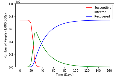
MatPlotLib graph for PJAS 2019 Measles example

It works! But as with all things, there are some problems. The first is that the SIR Model I chose to use lacks something called vital dynamics. Put simply vital dynamics are natural birth and death rates. The second is that it doesn’t take into account many factors such as autoimmune diseases, dietary differences, and so many other things that can vary the data. And third, any value we use for our recovery period or transmission rate will always be an average or a general number because diseases and humans are all different.

Overall this was one heck of a project, it was great fun to research into, and winning first place was a great bonus. My slides from the competition are attached on the new “Slides” page on the site. I’m working on many more projects this summer including some research with a college professor, so come back for that!

Thanks for reading and have a wonderful day!
~ Corbin

Leave a Reply